Bayesian Model Averaging

Basic Ideas

Assume we want to investigate some problem by statistical method, and we have data D. several possible statistical models are $M_1$, $M_2$…The number of models could be quite large. For example, if we consider only regression models but are unsure about which of $p$ possible predictors to include, there could be as many as $2^p$. BMA uses Bayesian statistics to select possible candidate predictors and help use construct the right model.

Methology Introduction

consider the unknown quantity of interest $\Delta$ and observed data $D$. we have possible models,$M_1$, $M_2$…$M_k$ , to do the estimation and forecasting. Then by a simple application of the
law of total probability, the BMA posterior distribution of $\Delta$ is

$p(\Delta | D)=\sum\limits_{k = 1}^K {p(\Delta |D,M_k)p(M_k|D)} \ \ (1)$

where $p(\Delta |D,M_k)$ is the posterior distribution of $\Delta$ given the model $M_k$, and $p(M_k|D)$ is the posterior probability that $M_k$ is the correct model, given that one of the models considered is correct. Thus the BMA posterior distribution of $\Delta$ is a weighted average of the posterior distributions of $\Delta$ under each of the models, weighted by their posterior model probabilities.(take the above equation as a weighted average case).

note that $p(\Delta |D,M_k)$ and $p(M_k|D)$ can be probability density functions, probability mass functions, or cumulative distribution functions.

The posterior model probability of $M_k$ is given by

$p(M_k|D) = \frac{p(D| M_k)p( M_k)} { \sum \limits_{l = 1}^K {p(D| M_l ) p(M_l)} } (2)$

$p(D| M_k)$ is the integrated likelihood of model $M_k$ , obtained by integrating (not maximizing)
over the unknown parameters

$p(D|M{k}) = \int p(D|\theta{k},M{k})p(\theta{k}|M{k}){\rm d}\theta{k}=\int (likelihood \times prior)\ {\rm d}\theta_{k}$

where $θ_k$ is the parameter of model $M_k$ and $p(D| \theta_k, M_k)$ is the likelihood of $\theta_k$ under model $M_k$ . The prior model probabilities are often taken to be equal, so they cancel in (2), but the BMA package allows other formulations also

information criterion

from the above (3), we see that the integrated likelihood $p(D| M_k )$ is a high dimensional integral that can be hard to calculate analytically. recalling the Maximum likelihood selection creteria, we found that $p(D| M_k )$ can be the simple and surprisingly accurate BIC approximation, which greatly simplify the model selection and calculation procedure

$2 \log p(D|M_{k})\approx2\log p(D|\tilde{\theta}_{k})-d_{k}\log(n)=-BIC_{k}$

where $d_{k}=\dim(\theta_{k})$ is the number of independent parameters in $M_k $, and $\tilde{\theta}_k$ is the maximum likelihood estimator (equal to the ordinary least squares estimator for linear regression coefficients).

And for linear regression, BIC has the simple form:

$BIC_{k}=n\log(1-R_{k}^{2})+p_{k}\log{n}$

up to an additive constant, where $R_k^2$ is the value of $R^2$ and $P_k$ is the number of regressors for the kth regression model.

eg: to illustrate what $\Delta$ is:

When interest focuses on a model parameter, say a regression parameter such as $\beta_1 $ , (1) can be applied with $\Delta =\beta_1$ . The BMA posterior mean of $\beta_1$ is just a weighted average of the posterior means of $\beta_1$ under each of the models:

$E[\beta_{1}|D]=\sum \hat{\beta}_{1} p(M_{k}|D)$

which can be viewed as a model-averaged Bayesian point estimator. $\hat{\beta}_{1}$ is the posterior mean of $\beta_1$ under model $M_k$, and this can be approximated by the corresponding maximum likelihood estimator, $\hat{\beta}_{1}$ (Raftery, 1995).

For a survey and literature review of Bayesian model averaging, see Hoeting et al. (1999)

Application

Linear REgression

we use the UScrime dataset on crime rates in 47 U.S. states in 1960 (Ehrlich, 1973); this is
available in the MASS library. There are 15 potential independent variables, all associated with crime rates in the literature. The last two, probability of imprisonment and average time spent in state prisons, were the predictor variables of interest in the original study, while the other 13 were control variables. All variables for which it makes sense were logarithmically transformed. The commands are:


library(BMA)
library(MASS)
data(UScrime)
x.crime<- UScrime[,-16]
y.crime<- log(UScrime[,16])
x.crime[,-2]<- log(x.crime[,-2])
crime.bicreg <- bicreg(x.crime, y.crime)
summary (crime.bicreg, digits=2)

 plot (crime.bicreg,mfrow=c(4,4)) # c(4,4) 意思是图形以4行4列共16个集体显示

This summary yields Figure 1. (The default number of digits is 4, but this may be more than
needed.) The column headed “p!=0” shows the posterior probability that the variable is in the model (in %). The column headed “EV” shows the BMA posterior mean, and the column headed “SD” shows the
BMA posterior standard deviation for each variable. The following five columns show the parameter estimates for the best five models found, together with the numbers of variables they include, their $R^2$ values, their BIC values and their posterior model probabilities.

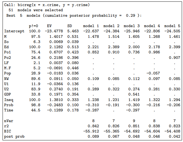
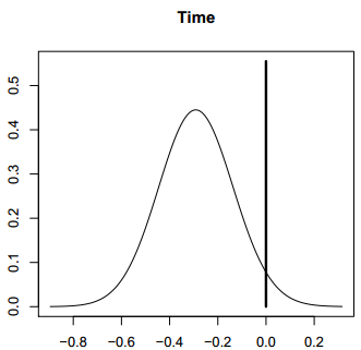
Figure 2: BMA posterior distribution of the coefficient of the average time in prison variable in the
crime dataset. The spike at 0 shows the posterior probability that the variable is not in the model.(在0点的那条竖线的纵坐标值代表不在模型中的概率是多少) The curve is the model-averaged posterior density of the coefficient given that the variable is in the model, approximated by a finite mixture of normal distributions, one for each model that includes the variable. The density is scaled so that its maximum height is equal to the probability of the variable being in the model.

Logistic Regression

We illustrate BMA for logistic regression using the low birthweight data set of Hosmer and Lemeshow
(1989), available in the MASS library. The dataset consists of 189 babies, and the dependent variable
measures whether their weight was low at birth. There are 8 potential independent variables of which
two are categorical with more than two categories: race and the number of previous premature labors
(ptl). Figure 5 shows the output of the commands


library(BMA)
library(MASS)
data(birthwt)
birthwt$race <- as.factor (birthwt$race)
birthwt$ptl <- as.factor (birthwt$ptl)
bwt.bic.glm <- bic.glm (low ~ age + lwt
+ race + smoke + ptl + ht + ui + ftv,
data=birthwt, glm.family="binomial")
summary (bwt.bic.glm,conditional=T,digits=2)

The function bic.glm in BMA can accept a formula, as here, instead of a design matrix and dependent variable (the same is true of bic.surv but not of bicreg)

Survival Analysis

BMA can account for model uncertainty in survival analysis using the Cox proportional hazards model.We illustrate this using the well-known Primary Biliary Cirrhosis (PBC) data set of Fleming and Harrington (1991). This consists of 312 randomized patients with the disease, and the dependent variable was survival time; 187 of the records were censored. There were 15 potential predictors. The data set is available in the survival library, which is loaded when BMA is loaded.

library(BMA)
library(MASS)
data(pbc)
x.pbc<- pbc[1:312,]
surv.t<- x.pbc$time
cens<- x.pbc$status
x.pbc<- x.pbc[,-c(6,7,10,17,19)]
x.pbc$bili<- log(x.pbc$bili)
x.pbc$alb<- log(x.pbc$alb)
x.pbc$protime<- log(x.pbc$protime)
x.pbc$copper<- log(x.pbc$copper)
x.pbc$sgot<- log(x.pbc$sgot)
pbc.bic.surv <- bic.surv(x.pbc,surv.t,cens)
summary(pbc.bic.surv,digits=2)
plot(pbc.bic.surv,mfrow=c(4,4))
imageplot.bma(pbc.bic.surv)

Summary

Based on R package BMA, we can easily deal with Bayesian model averaging for linear regression, generalized linear models, and survival or event history analysis using Cox proportional hazards models. More specific coding can refer to the manual of BMA. But based on the above knowledge, we are able to do some simple application by BMA.