Neural Network Tutorial
This note introduce the basic concept of neural network in machine learning, plus the python realization. this note is intended to tell beginners the cornerstone of the neural network and help anyone who is interested in neural network can build their own application easily.
The notes contains the following part:
- Toy example of Neural Network
- The Defination of Neural Network
- Bsic element in Neural Network and Backprogation
- constuct the Neural Network
Toy example
First Case
The example comes from @iamtrask, link blog
the toy example is neural network trained with backpropagation is attempting to use input to predict output.
| Inputs | Inputs | Inputs | Output |
|---|---|---|---|
| 0 | 0 | 1 | 0 |
| 1 | 1 | 1 | 1 |
| 1 | 0 | 1 | 1 |
| 0 | 1 | 1 | 0 |
we would see that the leftmost input column is perfectly correlated with the output. Backpropagation, in its simplest form.
| Variable | Definition |
|---|---|
| X | Input dataset matrix where each row is a training example |
| y | Output dataset matrix where each row is a training example |
| l0 | First Layer of the Network, specified by the input data |
| l1 | Second Layer of the Network, otherwise known as the hidden layer |
| syn0 | First layer of weights, Synapse 0, connecting l0 to l1. |
| * | Elementwise multiplication, so two vectors of equal size are multiplying corresponding values 1-to-1 to generate a final vector of identical size. |
| - | Elementwise subtraction, so two vectors of equal size are subtracting corresponding values 1-to-1 to generate a final vector of identical size. |
| x.dot(y) | If x and y are vectors, this is a dot product. If both are matrices, it’s a matrix-matrix multiplication. If only one is a matrix, then it’s vector matrix multiplication. |
1 | import numpy as np |
Output After Training:
[[ 0.00966498]
 [ 0.00786546]
 [ 0.99358866]
 [ 0.99211917]]
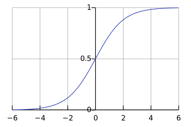
A sigmoid function maps any value to a value between 0 and 1. We use it to convert numbers to probabilities. It also has several other desirable properties for training neural networks.
A sigmoid function maps any value to a value between 0 and 1. We use it to convert numbers to probabilities. It also has several other desirable properties for training neural networks.
A Harder Problem XOR
The problem can be described in the following table :
| Inputs | Inputs | Inputs | Output |
|---|---|---|---|
| 0 | 0 | 1 | 0 |
| 0 | 1 | 1 | 1 |
| 1 | 0 | 1 | 1 |
| 1 | 1 | 1 | 0 |
The realized code is in the following and the definations of each variables are :
| Inputs (l0) | Inputs (l0) | Inputs (l0) | Hidden Weights (l1) | Hidden Weights (l1) | Hidden Weights (l1) | Hidden Weights (l1) | Output (l2) |
|---|---|---|---|---|---|---|---|
| 0 | 0 | 1 | 0.1 | 0.2 | 0.5 | 0.2 | 0 |
| 0 | 1 | 1 | 0.2 | 0.6 | 0.7 | 0.1 | 1 |
| 1 | 0 | 1 | 0.3 | 0.2 | 0.3 | 0.9 | 1 |
| 1 | 1 | 1 | 0.2 | 0.1 | 0.3 | 0.8 | 0 |
1 | import numpy as np |
Error:0.0085850250975
Error:0.00578962106435
Error:0.00462926115218
Error:0.0039588188244
Error:0.0035101602766
Error:0.00318353073559
decode the above program
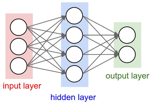
The above progam is acutally three nodes for input layer, four nodes for hidden layer (only 1 hidden layer) and 1 node output layer. we have four observational data. the number of weights (Synapses) need to calcualte is 3*4 + 1*4. For fiting the data, the code use traditional backprogation method to update the weightings and raise the prediction precise. When the code calculate the result, it needs to know the error to the training data. l2_error = y - l2 Then, based on the error distance, we can make the correction. Firstly, the last node, we want to know how to update the weights in the last layer. this is l2_delta = l2_error*nonlin(l2,deriv=True). After that, we need to know the how the error contribution contributed to the weights in the upper layer. Then, we need the backprogation method to calculate the extent of one unit change of the weights in the upper layer to final error. This can use derivates to express,
So we have l1_error = l2_delta.dot(syn1.T). In addition, we have l1_delta = l1_error * nonlin(l1,deriv=True)
The l1_delta and l1_delta indicate the update coefficients that weights should concern, multiplied by input value we can get the update amount of different weights in the Neural Network, which is the last two lines:
syn1 += l1.T.dot(l2_delta)
syn0 += l0.T.dot(l1_delta)
The Defination of Neural Network
Biological motivation
the online lecture notes have very clearly introduce to the neural network .(see note1)
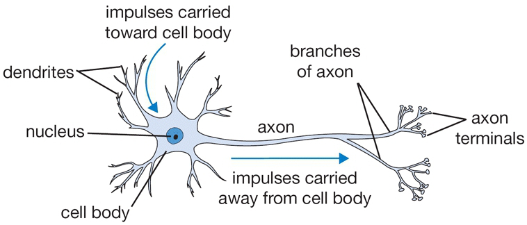
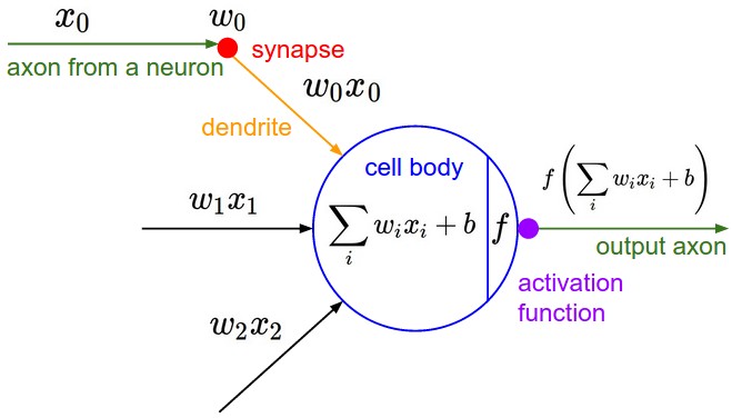
Here I briefly mention the basic ideas of eural network. The neural Network mimick human brain neurons performance. different neurons connect with each other by synapses, and receives the input signals from dendrites. In the nucleus, it applies activation function to produce the output singals, and then send the singal to the next neurons through its axon and synapses
The above description illustrate the functioning procedures of the very basic neural network.
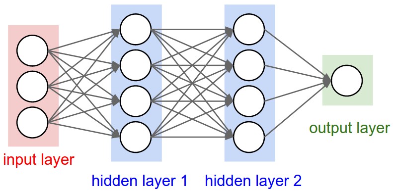
Neural Network architectures
Instead of an amorphous blobs of connected neurons, Neural Network models are often organized into distinct layers of neurons.
Self Understanding
As far as I learned in neural network, it can be seen as weighting different analysis core to produce the final judgement. for example, in one specific node at jth layer, it can receive all or part of input signal from upper layer. when it receive those signals, there are many ways to organzie them. the simplest way is liner form, multiplying them with weightings (synapses)(eg $w1x1+w2x2+w3x3$). But we could also apply other forms such as polynomial, quardatic form, max, … And when we do like this, we need to remember that we need to output singal. So we need to apply *activation function (usually sigmoid) to swith the numerical result into the singal. By combing many nodes and many layers, we can deal with many complex issues and get the desired results. I think this is the power of Neural Network. In Big Data era, Neural Network must have wider and wider applications.