Continuous Time Model

Abstract This notes is about the study of continuous time dynamic model based on “The Art of Smooth Pasting”

Brownian Motion

The Brownian Motion was first formulated to represent the motion of small particles suspended in a liquid. To decribe the motion, given the initial value $x_{0}$ at time $t=0$ , the random variable $x_{t}$ for any $t>0$ is normally distributed with mean $(x_{0}+\mu t)$ and variance $(\sigma^{2}t)$ . The parameter $\mu$ measures the trend , and $\sigma$ the volatility of the process. For the Brownian motion, $x_{t}$ as its ’position’, and a graph of $x_{t}$ against $t$ as its ’path’.

The infinitesimal random increment $dx$ over the infinitesimal time $dt$ having mean $\mu dt$ and variance $\sigma^{2}dt$. Just as we write normal random varible as $\mu+\sigma w$ where $w$ is a standard normal varible of $N(0,1)$, we can

$$dx=\mu dt+\sigma dw \tag{1}$$

where $w$ is a standardized Brownian motion (Wiener process) whose increment $dw$ has zeros mean and variance $dt$

The (Ito) Calculus of such infinitesimal random variables differs in some important ways from the usual non-random calculus. Since a fully rigorous treatment of ito calculus is quite difficult, a non-rigorous exposition should suffices for many economic applications. So here we can approximate Brownian motion by a discrete random walk. Then the normal distribution arises as the limit of a sum of independent binary variables $\bigtriangleup x$ over discret time intervals $\bigtriangleup t$ when these go to zero in a particular way.

Random Walk and Brownian Motion

This subsection try to bridge the discrete random walk with continuous Brownian motion. To do so, we can divide time into discrete period of length $\bigtriangleup t$, and $\bigtriangleup h$ can be seen as the step-length or the distance between successive points.

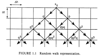
Let $\bigtriangleup x$ be a random variable that follows a random walk: in one time period it moves up one step in space with probability $p$, and one step down with probability $q=1-p$. Note: $\bigtriangleup h$ is given positive number, and $\bigtriangleup x$ is a random variable that takes values $\pm\bigtriangleup h$ . Figure 1.1 illustrate this with time marching downward and position shown horizontally. So the mean and variance of $\bigtriangleup x$ are

$$\begin{align} E[\bigtriangleup x] & =p\bigtriangleup h+q(-\bigtriangleup h)=(p-q)\bigtriangleup h \tag{2} \\ Var[\bigtriangleup x] & =E[(\bigtriangleup h)^{2}]-(E[\bigtriangleup x])^{2}\nonumber \\ & =4pq(\bigtriangleup h)^{2} \tag{3} \end{align}$$

A time interval of length $t$ has $n=t/\bigtriangleup t$ such discrete steps. Since the successive steps of the random walk are independent, the cumulated change $(x_{t}-x_{0})$ is a binominal variate with mean

$$n(p-q)\bigtriangleup h=(p-q)\bigtriangleup h\cdot t/\bigtriangleup t$$

and variance

$$4npq(\bigtriangleup h)^{2}=4pq(\bigtriangleup h)^{2}\cdot t/\bigtriangleup t$$

(Recall the relation between Bernoulli distribution and Binomial distribution) Remember the binomial distribution, a ’success’ in any one trial counts as 1 and occurs with probability p, while a failure counts as 0 and occurs with probability $q=1-p$. The (random) number of successes in $n$ independent trials has expectation $np$ and variance $npq$. So back to this problem, now the success counts as $\bigtriangleup h$ and failure as $-\bigtriangleup h$. Now set

$$\bigtriangleup h=\sigma\sqrt{\bigtriangleup t} \ \ (4)​$$

and

$$p=\frac{1}{2}[1+\frac{\mu}{\sigma}\sqrt{\bigtriangleup t}],\ \ q=\frac{1}{2}[1-\frac{\mu}{\sigma}\sqrt{\bigtriangleup t}] \ \ (5)$$

or

$$p=\frac{1}{2}[1+\frac{\mu}{\sigma^{2}}\sqrt{\bigtriangleup t}],\ \ q=\frac{1}{2}[1-\frac{\mu}{\sigma^{2}}\sqrt{\bigtriangleup t}]$$

Then

$$4pq=1-\left(\frac{\mu}{\sigma}\right)^{2}\bigtriangleup t$$

Substitute these into the above expression. and let $\bigtriangleup t$ go to zero. Then the Binomial distribution converges to the normal, with mean

$$t\frac{\mu}{\sigma^{2}}\bigtriangleup h\frac{\bigtriangleup h}{\bigtriangleup t}=\mu t$$

and variance $t[1-\left(\frac{\mu}{\sigma}\right)^{2}\bigtriangleup t]\frac{\sigma^{2}\bigtriangleup t}{\bigtriangleup t}\rightarrow\sigma^{2}t$

Thus we can regard Brownian motion as the limit of the random walk, when the time interval and the space step-ength go to zero together.

The mean of $(x_{t}-x_{0})$ is $\mu t$ and its standard deviation is $\sigma\sqrt{t}$. For large $t$, we have $\sqrt{t}\ll t$; in the long run, the trend is the dominant determinant of brownian motion. But for small $t$, we have $t\ll\sqrt{t}$, so volatility dominates in the short run.

Another manifestation of this volatility is seen by calculating the expected length of a path. We have

$$E(|\bigtriangleup x|)=\bigtriangleup h$$

so the total expectedd length of the path over time interval from $0$ to $t$ is

$$t\bigtriangleup h/\bigtriangleup t=t\sigma/\sqrt{\bigtriangleup t}\rightarrow\infty$$

as $\bigtriangleup t$ goes to zero. For small but finite $\bigtriangleup t$, the total length of almost all sample path is very large. Therefore each path must have many ups and sowns and look very jagged. Most such sample paths are not differentiable. When discussing the expected rate of change, therefore, we must write $E[dx]/dt$ not $E[dx/dt]$

Ito’s Lemma

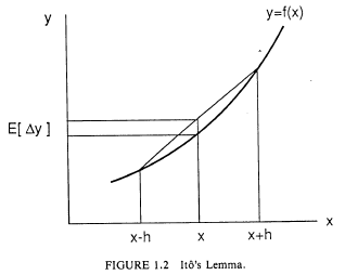
Suppose $x$ follows Brownian motion with parameters $(\mu,\sigma)$. Consider a stochastic process y that is related to $x$ by $y=f(x)$ where $f$ is a given non-random function. We want to related changes in y to those in x. The rules of conventional calculus suggest writing $dy=f’(x)dx$ and taking expectations. How the changes in x relate to changes in y ? The rules of conventional calculus suggest writing $dy=f’(x)dx$ and taking expectations. But this turns out to be wrong. The reason is as follows. Starting at $y_{0}=f(x_{0})$ , consider the position a small amount of time $t$ later.

$$y_{t}-y_{0}=f'(x_{0})(x_{t}-x_{0})+\frac{1}{2}f''(x_{0})(x_{t}-x_{0})^{2}+...$$

Hence

$$\begin{aligned} E[y{t}-y{0}] & =f'(x{0})E[x{t}-x{0}]+\frac{1}{2}f^{''}(x{0})E[(x{t}-x{0})^{2}]+...\\ & =f'(x{0})\mu t+\frac{1}{2}f^{''}(x{0})[\sigma^{2}t+\mu^{2}t^{2}]+...\\ & =[\mu f'(x{0})+\frac{1}{2}\sigma^{2}f^{''}(x{0})]t+...\end{aligned}$$

Note that the second order term in the Taylor expansion of $f(x)$ contributes a term that is not ignorable. The reason is that the variance of the increments of $x$ is linear in t. This is the feature that makes the calculus of Brownian motion so different from the usual calculus of non-random variables. A similar calculation will show that

$$Var[y_{t}-y_{0}]=f'(x_{0})^{2}\sigma^{2}t+...$$

Let $x$ denote a general starting and $y=f(x)$. Consider the infinitesimal increment $dy$ over the next infinitesimal time interval $dt$. We can use the above expression replacing $t$ with $dt$ and ignoreing higher order terms in $dt$. Therefore $dy$ has mean

$$E[dy]=[f^{'}(x)\mu+\frac{1}{2}f^{''}(x)\sigma^{2}]dt$$

and variance

$$Var[dy]=f'(x)^{2}\sigma^{2}dt$$

So $y$ follows the general diffusion process defined by

$$dy=[f'(x)\mu+\frac{1}{2}f^{''}(x)\sigma^{2}]dt+f'(x)\sigma dw \ \ (6)$$

This is Ito Lemma in the form that will prove most useful for the study. A slight generalization is easily available : if $y=f(x,t)$, the Taylor expansion has an addition term in $f_{t}$, and

$$dy=[f_{x}(x,t)\mu+\frac{1}{2}f_{xx}(x,t)\sigma^{2}+f_{t}(x,t)]dt+f_{x}(x,t)\sigma dw \ \ (7)$$

For a simple intuition, return to the discrete random walk formulation, and suppose $x$ ahs zeros trend, so $p=q=\frac{1}{2}$. Now $E[\bigtriangleup x]=0$ and as time passes the distribution of $x$ merely spreads out with linearly increasing variance around an unchanging mean. From the standard intution of risk -aversion , or Jensen’s inequality, we know the sign of $E[\bigtriangleup y]$ will be negative if $f$ is concave and positive if $f$ is convex.

GEometric Brownian motion

Now suppose x follows the Brownian motion, and let $X=e^{x}$. Ito’s Lemma gives

$$E[dX]=[e^{x}\mu+\frac{1}{2}e^{x}\sigma^{2}]dt=X[\mu+\frac{1}{2}\sigma^{2}]dt$$

and $Var(dX)=[e^{x}]^{2}\sigma^{2}dt=X^{2}\sigma^{2}dt$

Therefore the process of $X$ can be written

$$dX/X=[\mu+\frac{1}{2}\sigma^{2}]dt+\sigma dw$$

This is called the geometric or proportional Brownian motion. It provides a good first approximation of the dynamics of exchange rates, prices of natural resources, and more generally many asset prices.

Conversely, if $X$ follows the geometric Brownian motion

$$dX/X=vdt+\sigma dz \ \ (8)$$

then using Ito’s Lemma we find that $x=\ln X$ follows the ordinary or absolute Brownian motion

$$dx=[v-\frac{1}{2}\sigma^{2}]dt+\sigma dw$$

Notice that $d\text{\ensuremath{\ln}}x\neq dX/X$ . Suppose $X$ follows geometric Brownian motion (8) with the known position $X_{0}$ , with the relation of $x=\ln X$ we finally can get

$$E(X_{t})=\exp(x_{0}+\mu t+\frac{1}{2}\sigma^{2}t)=X_{0}e^{vt}$$

Since exponential is a convex function, therefore

$$E[X_{t}]=E[\exp x_{t}]>\exp E[x_{t}]=\exp(x_{0}+\mu t)$$

Some generalizations

If the trend and volatility coefficients are functions of the current state ($x$), this is often called a diffusion process.When they are functions of time as well, it is sometimes called an Ito process.

$$dx=\mu(x,t)dt+\sigma(x,t)dw \ \ (9)$$

By the defintion of diffiusion process, we can see that (8) geometric brownian motion is a special case of diffusion process

$$dX=\mu Xdt+\sigma Xdw$$

In come cases, we may need processes that revert toward some central level $\bar{x}$ of the state variable

$$dx=-\theta(x-\bar{x})dt+\sigma dw \ \ (10)$$

where $\theta$ is some positive constant.

Also, several variabes $x_{i}$ for $i=1,2,..m$ may follow Brownian motion, their volatility components being linear combinations of independent standard Wiener processes $w_{j}$ for $j=1,2,…n$

$$dx_{i}=\mu_{i}dt+\sum_{j=1}^{n}a_{ij}dw_{j}$$

Then

$$\begin{aligned} E[dx{i}] & =\mu{i}dt \\ Var[dx_{i}] &=\sum_{j=1}^{n}(a{ij})^{2}dt \\ Cov[dx_{i},dx_{k}]&=\sum_{j=1}^{n}a_{ij}a_{kj}dt \end{aligned}$$

Such multi-variable processes are important in financial economics.

Discounted Present Values

Now we can move to some real economic examples. First let’s consider an economic unit, such as a firm , in a dynamic stochastic setting. Its state at time $t$ is given by a state variable $x_{t}$ that follows a Brownian motion with exogenous parameters $\mu$ and $\sigma$. There is a net flow payoff $f(x_{t})$ , such as profit or dividend, that depends on the state $x_{t}$. The expected present value $F(x)$ of the payoff starting at a given initial position $x_{0}=x,$and using an exogenously specified discout rate $\rho$, is defined by

$$F(x)=E\{\int_{0}^{\infty}f(x_{t})e^{-\rho t}dt|x_{0}=x\} \ \ (11)$$

Ultimately we will be interested in controlling or regulating the motion of $x_{t}$to optimize such expected present values net of the cost of control. To this end, we begin by evaluating $F(x)$ explicitly when $f(x)$ has some particularly simple functional forms such as exponentials and polynomial. Then we can get power series expression for $F(x)$ when $f(x)$ is any analytic function.

Prensent value for exponential and polynomials

First we conside the special case when the flow payoff has the form

$$f(x)=\exp(\lambda x)$$

The discounted present value $F(x)$ will be finite when $\lambda$ is in a certain range. Starting from the initial value $x_{0}=x$ , $x_{t}$ at time $t$ has a normal distribution with mean $(x+\mu t)$ and variance $\sigma^{2}t$. Then

$$E[exp(\lambda x_{t})|x_{0}=x]=\exp[\lambda(x+\mu t)+\frac{1}{2}\lambda^{2}\sigma^{2}t]$$

How to get the above expression, Here is the illustrative example. Suppose a random variable $x$ is normal with mean$m$and std $s$

$$\begin{aligned} E[\exp(\lambda x)] & =\frac{1}{s\sqrt{2\pi}}\int_{-\infty}^{\infty}\exp(\lambda x)\exp\left[-\frac{(x-m)^{2}}{2s^{2}}\right]dx\nonumber \\ & =\frac{\exp(\lambda m)}{s\sqrt{2\pi}}\int_{-\infty}^{\infty}\exp(\lambda y-\frac{y^{2}}{2s^{2}})dy\ y=x-m\nonumber \\ & =\frac{\exp(\lambda m+\frac{1}{2}\lambda^{2}s^{2})}{s\sqrt{2\pi}}\int_{-\infty}^{\infty}\exp\left[-\frac{(y-\lambda s^{2})^{2}}{2s^{2}}\right]dy\nonumber \\ & =\exp[\lambda m+\frac{1}{2}\lambda^{2}s^{2}] \ \ (12) \end{aligned}$$

Now we have the present value of$F(x)$

$$\begin{aligned} F(x) & =\int{0}^{\infty}E[exp(\lambda x{t})|x_{0}=x]\exp(-\rho t)dt\nonumber \\ & =\exp(\lambda x)\int_{0}^{\infty}\exp[\lambda\mu t+\frac{1}{2}\lambda^{2}\sigma^{2}t]dt\nonumber \\ & =\exp(\lambda x)/(\rho-\lambda\mu-\frac{1}{2}\lambda^{2}\sigma^{2}) \ \ (13) \end{aligned}$$

The intergal converges provided the denominator is positive. To describe the convergence property, it is useful to give a uniforma notation and interpretation at the outset.

$$\phi(\xi)=\rho-\xi\mu-\frac{1}{2}\xi^{2}\sigma^{2} \ \ (14)$$

Labed as the Fundamental Quadratic of Brownian Motion

The condition for the convergence of the integral in (11) amounts to requiring that $\lambda$lies in the interval $(-\alpha,\beta)$ This includes $\lambda=0$ .

We can use the formula 11 to derive an expression for $F(x)$ when $f(x)$ in any integer power $x^{n}$. For exponential flow function

$$\begin{matrix} F(x) & =E[\int_{0}^{\infty}\sum_{n=0}^{\infty}\frac{1}{n!}(\lambda x{t})^{n}e^{-\rho t}dt|x_{0}=x]\\ & =\sum_{n=0}^{\infty}\frac{\lambda^{n}}{n!}E[\int_{0}^{\infty}x{t}^{n}e^{-\rho t}dt|x_{0}=x] \end{matrix}$$ $$\begin{aligned} \exp(\lambda x) & =\sum_{k=0}^{\infty}\frac{1}{n!}\lambda^{n}x^{n}\\ [\rho-\mu\lambda-\frac{1}{2}\sigma^{2}\lambda^{2}]^{-1} & =\frac{1}{\rho}\sum_{n=0}^{\infty}\rho^{-n}(\mu\lambda+\frac{1}{2}\sigma^{2}\lambda^{2})^{n} \end{aligned}$$

For each power of $x​$ we write out first two, and rest follows same tedious calcualtion

$$\begin{aligned} E\{\int_{0}^{\infty}x{t}e^{-\rho t}dt \} & =\frac{\mu}{\rho^{2}}+\frac{x}{\rho} \ \ (15) \\ E\{ \int_{0}^{\infty}x{t}^{2}e^{-\rho t}dt \} & =[\frac{\sigma^{2}}{\rho^{2}}+\frac{2\mu^{2}}{\rho^{3}}]+\frac{2\mu x}{\rho^{2}}+\frac{x^{2}}{\rho} \ \ (16) \end{aligned}$$

Finally consider any analytic $f(x)$ with the power series representation

$$f(x)=\sum_{n=0}^{\infty}f_{n}(x^{n})$$

assumed uniformly convergent for all $x$. Having found the expected present values of all integer powers, we can integrate term by term to find the $F(x)$ corresponding to this analytic $f(x)$. Thus we can in-principle complete the calculation of present values for most common functions of Brownian motion.

Present values for powers of geometric Brownian motion

Next suppose $X$ follows the geometric brownian motion,

$$dX/X=vdt+\sigma dw$$

We want to find the expected present value when flow payoff is $g(X)=X^{\lambda}$. Note that $x=\ln(X)$ follows the Brownian motion

$$dx=(v-\frac{1}{2}\sigma^{2})dt+\sigma dw$$

and $X^{\lambda}=\exp(\lambda x)$ , we have

$$\begin{aligned} E{\int_{0}^{\infty}X_{t}^{\lambda}e^{-\rho t}dt} & =\exp(\lambda x)/[\rho-(v-\frac{1}{2}\sigma^{2})\lambda-\frac{1}{2}\sigma^{2}\lambda^{2}]\\ & =X^{\lambda}/[\rho-v\lambda-\frac{1}{2}\sigma^{2}\lambda(\lambda-1)] \ \ (17) \end{aligned}$$

The above will converge as long as denominator is positive. So the convergence condition is now defined as

$$\psi(\xi)=\rho-v\xi-\frac{1}{2}\sigma^{2}\xi(\xi-1) \ \ (18)$$

two economically natural assumption that $\rho>0$ and $\rho>v$ guarantee the roots of above equation $-\gamma<0$ and="" $\delta="">1$ . Similarly, $\lambda$ should lie in the interval $(-\gamma,\delta)$.

For $Y=X^{\lambda}$, we have

$$dY/Y=[\lambda v+\frac{1}{2}\lambda(\lambda-1)\sigma^{2}]dt+\lambda\sigma dw$$

For the convergence of the expected present value of $Y$, the discount rate must exceed the trend growth rate of $Y$ which is $\psi(\lambda)>0$ And for the relation between absolute and geometric Brownian motion, if $x=\ln X$, we have that $\mu=v-\frac{1}{2}\sigma^{2}$

$$\begin{aligned} \psi(\xi) & =\rho-(\mu+\frac{1}{2}\sigma^{2})\xi-\frac{1}{2}\sigma^{2}\xi(\xi-1)\\ & =\rho-\mu\xi-\frac{1}{2}\sigma^{2}\xi^{2} \\ & =\phi(\xi)\end{aligned}$$

And then the roots will also correspond ,with $\alpha=\gamma$ and $\beta=\delta$

A basic differential equation for present value

Now let us return to absolute Brownian motion $x$ and the flow payoff $f(x)$ , and consider an alternative characterization of the expected present value $F(x)$. Here we just want to use an alternative method to split the $F(x)$ integral into the contribution over the initial infinitesimal time interval from $0$ to $dt$ and the integral from $dt$ to $\infty$. Why we want to do this? Because through this we can get basic differential equation for $F(x)$

Note that start from $x+dx$ we need take discount value back to time $t=0$ . So we have

$$F(x)=f(x)dt+e^{-\rho dt}E[F(x+dx)]$$

Note that this is already an approximation in regarding $f(x)$ as constant over the small interval $dt$. the resulting error in $f(x)dt$ is of order $dt^{2}$. We further simplify the expression and get

$$\begin{aligned} F(x) & =f(x)dt+(1-\rho dt)(F(x)+[E[F(x+dx)]-F(x)])\\ & =f(x)dt+F(x)-\rho F(x)dt+[E[F(x+dx)]-F(x)] \end{aligned}$$

Therefore

$$\begin{aligned} \rho F(x)dt & =f(x)dt+[E[F(x+dx)]-F(x)]\nonumber \\ & =f(x)dt+E[dF] \ \ (19) \end{aligned}$$

The above is the arbitrary equation. Think of the entitlement to the flow payoffs as a capital asset; $F(x)$ is its value. Contemplate holding this asset over the period $(t,t+dt)$. This yields a dividend $f(x)dt$, and an expected capital gain $E[dF]$. The sum of these two should equal the normal return $\rho F(x)dt$

By Ito Lemma, (previous) $E[dF]=\mu F^{'}(x)dt+\frac{1}{2}\sigma^{2}F^{''}(x)dt$

Substituting into (15) and dividing by $dt$, we get

$$\frac{1}{2}\sigma^{2}F^{''}(x)+\mu F^{'}(x)-\rho F(x)+f(x)=0 \ \ (20)$$

Derivation by discrete approximation

We regarded Brownian motion as the limit of a discrete random walk, and we can also derive the differential equation (16) by that approach.

Label the discrete points in the $x$ space by $i$ , and the discrete time periods by $j$. Let $i_{j}$ denote the position of the particle at time $j$; future positions are of course random variables given our initial information at $j=0$. Then the expected present value can be written as

$$F(i)=E\left\{ \sum_{j=0}^{\infty}f(i_{j})\bigtriangleup te^{-j\rho\bigtriangleup t}|i_{0}=i\right\}$$

After the first step, the same problem restarts with a new initial state $i_{1}$, which from the time $0$ perspective can be either $(i+1)$ with probability $p$ or $(i-1)$ with probability $q$. Thus the expectation on the right hand side becomes

$$F(i)=f(i)\bigtriangleup t+e^{-\rho\bigtriangleup t}[pF(i+1)+qF(i-1)]$$

Now expand the right hand side, ignoring terms of higher order than $\bigtriangleup t.$ Note that

$$e^{-\rho\bigtriangleup t}=1-\rho\bigtriangleup t+...$$

Next , we reuse the definite of (5) of $p$ and $q$ and the relation (4) between the stepsize $\bigtriangleup h$ and the time interval $\bigtriangleup t$ we can get

$$\begin{aligned} pF(i+1)+qF(i-1) & =\frac{1}{2}[1+(\mu/\sigma)\sqrt{\bigtriangleup t}]F(x+\bigtriangleup h)\\ & \ \ +\frac{1}{2}[1-(\mu/\sigma)\sqrt{\bigtriangleup t}]F(x-\bigtriangleup h)\\ & =\frac{1}{2}[1+(\mu/\sigma)\sqrt{\bigtriangleup t}][F(x)+F^{'}(x)\bigtriangleup h\\ & \ \ +F^{''}(x)(\bigtriangleup h)^{2}+... ] \\ & =\frac{1}{2}[1+(\mu/\sigma)\sqrt{\bigtriangleup t}][F(x)-F^{'}(x)\bigtriangleup h+\\ & \ \ +F^{''}(x)(\bigtriangleup h)^{2}+... ] \\ & =F(x)+\mu F^{'}(x)\bigtriangleup t+\frac{1}{2}\sigma^{2}F^{''}(x)\bigtriangleup t+...\end{aligned}$$

Substituting and simplifying yield the same equation (the above equation) as (16)

$$F(i)=f(i)\bigtriangleup t+e^{-\rho\bigtriangleup t}+[1-\rho\bigtriangleup t][...]$$

The general solution

This part tells how to solve the second order differential equation. The differential equation (16) is linear. Therefore its general solution is the sum of two parts: any solution of the equation as a whole (particular integral) and the general solution of the homogeneous part of the equation with the term $f(x)$ omitted (the complementary function)¹.

To find the complementary function, write the homogeneous part of the equation:

$$\frac{1}{2}\sigma^{2}F^{''}(x)+\mu F^{'}(x)-\rho F(x)=0$$

Its general solution can be expressed as a linear combination of two independent solution. For instance, if we try solutions ofthe form $\exp(\xi x),$we get $\exp(\xi x)[\frac{1}{2}\sigma^{2}\xi^{2}+\mu\xi-\rho]=0$

Since the exponential is always positive, this holds if and only if

$$\frac{1}{2}\sigma^{2}\xi^{2}+\mu\xi-\rho=0$$

This is just $\phi(\xi)$ introduced above. So $\xi$ must equal $-\alpha$ or $\beta$ the two roots. The two roots are distinct. They have opposite signs. The two solutions $e^{-\alpha x}$and $e^{\beta x}$ are independent and the general solution is

$$Ae^{-\alpha x}+Be^{\beta x} \ \ (21)$$

where $A$ and $B$ are undetermined constants.

Finding a particular solution to the full equation (16) is often an art (with lucky) , but for the exponential and polynomial forms we tried before, there are obvious choice.

Begin with the exponential case. When $f(x)=exp(\lambda x)$ the form $F(x)=K\exp(\lambda x)$ suggest itself

$$K(\frac{1}{2}\sigma^{2}\lambda^{2}+\mu\lambda-\rho)\exp(\lambda x)+\exp(\lambda x)=0$$

we get $K=1/\phi(\lambda)$

Combining this particular solution and the earlier complementary function, the general solution for the expected present value in the exponential case becomes

$$F(x)=\frac{1}{\phi(\lambda)}e^{\lambda x}+Ae^{-\alpha x}+Be^{\beta x} \ \ (22)$$

In fact, a simple argument shows that when the flow $f(x)$ is the exponential $exp(\lambda x)$ the expected present values $F(x)$ must be a multiple of $\exp(\lambda x)$. To give a formal argument, define $y_{t}=x_{t}-h$ and consider the stochastic process $y_{t}$

$$dy=dx=\mu dt+\sigma dw$$

and the initial position $y_{0}=(x+h)-h=x$. The flow benefit can be written

$$F(x+h)=e^{\lambda x_{t}}=e^{\lambda h}e^{\lambda y_{t}}=e^{\lambda h}f(y_{t})$$

Integrating over time and taking expectation, we get

$$F(x+h)=e^{\lambda h}E\left\{ \int_{0}^{\infty}f(y_{t})e^{-\rho t}dt|y_{0}=x\right\}$$

Subtracting $F(x)$ from both side, dividing by $h$, and letting $h$ go to zero, we get

$$\lim_{h\rightarrow0}\frac{F(x+h)-F(x)}{h}=\lim_{h\rightarrow0}\frac{\exp(\lambda h)-1}{h}F(x)$$

or

$$F^{'}(x)=\lambda F(x)$$

As we can see the genral solution above was a combination of three terms, of which only the first, corresponding to the particular solution we guessed initially, had the right exponential form. Both $A$ and $B$ are zero. In the same way we can guess similar form of functions.

Now consider the polynomial case. When $f(x)=x^{n}$ for a positive integer $n$ , a natural guess for the particular integral is

$$F(x)=\sum_{m=0}^{n}a_{m}x^{m} \ \ (23)$$

Substituting this in $16$ we can get

$$\begin{aligned} \frac{1}{2}\sigma^{2}\sum_{m=2}^{n}m(m-1)a_{m}x^{m-2}+\mu\sum_{m=1}^{n}ma_{m}x^{m-1} \\ -\rho\sum_{m=0}^{n}a_{m}x^{m}+x^{m} & =0\end{aligned}$$

Collecting like powers of $x​$ together and equating the coefficient of each separately to zero since the equation must hold as an identity in $x​$ , we find

$$a_{n}=\frac{1}{\rho},a_{n-1}=n\mu/\rho^{2}$$

and for $m=0,1,2,…(n-2)$ the recursive relation

$$\rho a_{m}=(m+1)\mu a_{m+1}+\frac{1}{2}(m+1)(m+2)\sigma^{2}a_{m+2} \ \ (24)$$

This determines all the coefficients $a_{m}​$. Once again we can verify that the expected present value cannot have any contribution from the exponential of the complementary function. So (18) is the full solution.

Differential equation for the geometric Brownian motion

Now we turn again to geometric Brownian motion. Given a flow cost function $g(X)$, we want to find

$$G(X)=E\left\{ \int_{0}^{\infty}g(X_{t})e^{-\rho t}dt|X_{0}=X\right\} \ \ (25)$$

Proceeding exactly as before, we get the arbitrage equation

$$pG(X)dt=g(X)dt+E[dG]$$

and Ito Lemma gives

$$E[dG]=vXG'(X)dt+\frac{1}{2}(\sigma X)^{2}G^{''}(X)dt$$

Therefore the basic differential equation for the case of geometric Brownian motion is

$$\frac{1}{2}\sigma^{2}X^{2}G^{''}(X)+vXG^{'}(X)-\rho G(X)+g(X)=0 \ \ (26)$$

The complementary function is easily seen to be

$$CX^{-\gamma}+DX^{\delta} \ \ (27)$$

The same argument as before. Once agian the particular integral must be guessed. Previously we considered $g(X)=X^{\lambda}$ and natural guess for this is $G(X)=KX^{\lambda}$. Substituting into (20) we find

$$K=1/\psi(\lambda)$$

where $\psi(\lambda)$ is the fundamental quadratic for the geometric case. An argument similar to what we made above, the full solution is jsut the particular integral we guessed ; $C$ and $D$ are both zero.

We can change variables to transform geometric Brownian motion into an absolute one, and this gives an alternative way to find expected present values. Define $x=\ln X$ and $\mu=v-\frac{1}{2}\sigma^{2}$ . Let $f(x)=g(e^{x})$ $G(X)=F(\ln(X))$ . We will

$$F'(x)=e^{x}G'(e^{x})=XG'(X)$$

and

$$F^{''}(x)=(e^{x})^{2}G^{''}(e^{x})+e^{x}G^{'}(e^{x})=X^{2}G^{''}(X)+XG^{'}(X)$$

Substitution in (16) we find

$$0=\frac{1}{2}\sigma^{2}X^{2}G^{''}(X)+vXG^{'}(X)-\rho G(X)+g(X)$$

which is just (20). The two approaches are mutually consistent.

General diffusion process

If X follows the general diffusion process (9) rather than the simple Brownian motion (1), the expected value function $F(x)$ and the flow function $f(x)$ are linked by a differential equation that is a natural generalization of (16) namely

$$\frac{1}{2}\sigma(x)^{2}F^{''}(x)+\mu(x)F^{'}(x)-\rho F(x)+f(x)=0 \ \ (28)$$

Unfortunately, this time the solution is not the corresponding simple. The complementary function is specific to each case depending on the functional form of $\mu(x)$ and $\sigma(x)$. Analytical solution is possible only in very special cases. The geometric case was discussed above. for linearly mean-reverting motion (10) a power series solution related to the Confluent Hypergeometric function is avaibale; an example is developed in 5.1 .

If $x$ follows the Ito process (9) whose parameters depend on time as well as the state $x$, or if the flow payoff is a function $f(x,t)$ like wise, or the process ends at a given time $T$ so the time remaining to the end of the horizon matters, then we must allow the expected present value to depend on time too. The basic equation becomes a partial differential equation

$$\frac{1}{2}\sigma(x,t)^{2}F_{xx}(x,t)+\mu(x,t)F_{x}(x,t)-\rho F(x,t)+F_{t}(x,t)+f(x,t) \ \ (29)$$

The solution of this is much hard, and typically needs numerical methods.

Barriers

The above discussion assumed that the Brownian motion particle $x$ (absolute case) was free to range over the entire real line $(-\infty,+\infty)$. Similarly, in the case of geometric Brownian motion $X$ could range over $(0,\infty)$. In practice there are restrictions on the range. For example the output price facing one firm in a competitive industry is bounded above, because new firm will enter if the price rises beyond a certain point. Other cases the restrictions are exogenously imposed, as in the case of a government-imposed agricultural price floor. Finally, and most important for our purpose here, the restrictions arise endogenously through purposive optimal control of the stochastic propose.

In this section, the book will start with some specified restrictions on the process, and show how their effects on expected present values can be computed. The restrictions are called barriers. They can constrain upward or downward movement of $x$ , and are of two types, absorbing and reflecting.

at $b$ means that the process $(1)$ is allowed to proceed unhindered so long as $x_{t}<b$, but if ever $x_{t}=b$, the process is terminated. That might be the end of our planning horizon, or merely the end of the movement of $x$, so that it remains at $b$ for ever after. Sometimes such an absorbed process might be immediately restarted at a point $c<b$. Lower and two sided absorbing barriers are defined in obvious ways.

at $b$ means that the process $(1)$ is allowed to proceed unhindered so long as $x_{t}<b$, but if ever $x_{t}=b$, and the next increment $dx$ is positive, then the sign of this increment is reversed, as if the particle were reflected in a mirror placed at $b$. Once again, lower and two-sided barriers are defined analogously. We can even have an absorbing barrier on one side and a reflecting barrier on the other side.

Now consider a process with barriers for $x$, take a flow payoff function $f(x)$, and define the expected present value function $F(x)$ as in (20). When there wre no barriers, we took two approaches to finding $F(x)$. The first approach was direct. The distribution of $x_{t}$ given $x_{0}$ was known and simple, namely normal, so expected values of functions of $x_{t}$ could be found relatively easily. When there are barriers, between the starting time $0$ and the instant in question $t$ the particle might have been reflected at barriers any numer of times, or been absorbed with positive probability. The distribution of $x_{t}$ conditional on $x_{0}$ is much more complicated. This would be discussed in section 6.3. The second and indirect approach proves simpler. We show that $F(x)$ satisfies the same basic differential equation in the interior of the region of variation of $x$, and certain end-point conditions at the barriers. Finding $F(x)$ then amounts to solving the differential equations subject to the end-point conditions.

Basic differential equation

Suppose the process moves between barriers located at $a$ and $b$. For the moment it makes no difference whether the barriers are reflecting or absorbing, and $a=-\infty,b=\infty$ are permissible. Choosing the initial point $x_{0}=x$ in the interior of the range $[a,b]$. Over an infinitesimal time interval $dt$ , the probability of $x_{t}$, reaching either barrier is negligible. Therefore the arbitrage argument of section 2.3 remains valid, and the basic differential equation (20) holds. The derivation of section 2.4, based on discretization of the $x$ space, is also valid so long as the length of each step $\bigtriangleup h$ is chosen sufficiently small.

Even when the process has barriers, the flow function $f(x)$ is genrally defined over the full unrestricted range $(-\infty,+\infty)$ of the $x$ space. Even if it is not, we can extend its definition in some simpleway over the full range. Let $F_{0}(x)$ denote the expected present value of $f(x_{t})$ as defined in 2.1 above, and computed ignoring the barriers. Then we can follow previous procedure to calculate $F_{0}(x)$ for any analytic functions $f(x)$.

Our choice of $F_{0}(x)$, the expected present value ignoring barriers, as the particular integral gives a very nnice economic interpretation to the solution. Since the particular integral is what the expected present value would have been in the absence of barriers, the remaining part, namely the complementary function, must equal the effect of the barriers. For example, a price ceiling cuts off the upside profit potential of a firm; its effect is simply captured by the appropriate term in the complementary function. This actually tells us that it is the complementary function that exercise such control.

Recalling the form (21) of the complementary function.

$$F(x)=F_{0}(x)+Ae^{-\alpha x}+Be^{\beta x} \ \ (30)$$

The constants $A$ and $B$ must be determined using some other conditions on the problem. This is where the barriers come into play.

If $x$ is free to range over the entire line $(-\infty,+\infty)$ , we already know that $F(x)=F_{0}(x)$. Then $A$ and $B$ must both be zero.

If $x$ is not restricted on the lower side, but has an upper barrier at $b$, then we can get some information by considering what happens for very large negative values of $x$. Starting from such a value, the particle is unlikely to reach $b$ in any reasonable future time. Then the unrestricted expected present value $F_{0}(x)$ should be a good approximation for $F(X)$. But with $\alpha>0,\ e^{-\alpha x}$ goes to $\infty$ as x goes to $-\infty$. This would spoil the desired approximation unless $A=0$. Thus we have determined one of the constants. The other, $B$, is fixed using end-point conditions at the barrier $b$, which we will examine shortly.

Similarly, if $x$ has a only lower barrier at $a$, then the inspection of $F(x)$ as $x$ goes to $\infty$gives $B=0$, while $A$ is fixed by conditions at the barrier. If there are barriers on both sides, then both $A$ and $B$ are fixed by the end-point conditions at the barriers.

Geometric Brownian motion

Now suppose the underling variable is $X$, and it follows the proportional or geometric Brownian motion 1.8, with barriers at $c$ and $d$. Let the flow function be $g(X)$. Extending its definition outside the bariers to the full range $(0,\infty)$ of $X$ if necessary, following the similar setup as above 3.1, let $G_{0}(X)$ satisfies the basic differential equation 2.16 for geometic Brownian motion, and serves as a particular integral over the restricted range $(c,d)$ Then general solution is

$$G(X)=G_{0}(X)+CX^{-\gamma}+DX^{\delta} \ \ (31)$$

$-\gamma$ and $\delta$ are the roots of the fundamental quadratic (27), and $C,D$ are constants to be determined by conditions that apply at the barriers .

Stopping

Now let us return to the case of absolute Brownian motion, and begin the analysis of barriers, starting with an upper absorbing barrier.Suppose the barrier is placed at $b$. To set the stage for subsequent analysis of control, allow an exogenous terminal payoff $W(b)$. If x stays for ever at b after absorption, $W(b)$ may simply be the capitalized value of the constant flow payoff, $f(b)/\rho$. But other interpretations are also possible. If a cost $k$ must be paid at the instant of absorption, we simply subtract if from $W(b)$ to make it $W(b)-k$.

The expression (2.1) for the expected present value must be modified to take account of the barrier and the terminal payoff.

$$F(X)=E\left\{ \int_{0}^{t(b)}f(x_{t})e^{-\rho t}dt+e^{-\rho(b)}W(b)|x_{0}=x\right\} \ \ (32)$$

where $t(b)$ is the first time the process reaches $b$ starting at $x$, and of course it is a random variable given the initial information.

To find the conditions that hold at the barrier, we repeat the arbitrage calculation, but now starting at or near the barrier rather than at an interior point. Revert to the discrete approximation to Brownian motion, with time intervals $\bigtriangleup t$ and steps of length $\bigtriangleup h$. Starting at $(b-\bigtriangleup h)$, we have

$$F(b-\bigtriangleup h)=f(b-\bigtriangleup h)\bigtriangleup t+(1-\rho\bigtriangleup t)[pW(b)+qF(b-2\bigtriangleup h)]$$

Expanding the Taylor series, we get

$$\begin{aligned} F(b)-F'(b)\bigtriangleup h+... & =f(b)\bigtriangleup t+...+\frac{1}{2}W(b)[1-\rho\bigtriangleup t+...]\\ & +\frac{1}{2}(1-\rho\bigtriangleup t)[F(b)-2F'(b)\bigtriangleup h+...]\end{aligned}$$

Collecting terms, dividing by $\bigtriangleup h$ and taking limits, we find

$$F(b)=W(b) \ \ (33)$$

This is sometimes called the Value Matching condition.

Resetting

Here the process is allowed to follow (1.1) so long as $x<b$, but the instant $x$ hits $b$, it is reset at $x=c<b$, and the process is restarted. The calculation is as above, except that $F(c)$ replace $W(b)$, and we get a value matching condition $F(c)$ replaces $W(b)$, and we get a value matching condition $F(b)=F(c)$ . If the resetting entailed a cost $k$, this would become $F(b)=F(c)-k$

Reflection

Finally, suppose the process is reflected at an upper barrier $b$. Now starting at $b$ we are sure to go to $(b-\bigtriangleup h)$, so

$$\begin{aligned} F(b) & =f(b)\bigtriangleup t+(1-\rho\bigtriangleup t)F(b-\bigtriangleup h)\\ & =f(b)\bigtriangleup t+(1-\rho\bigtriangleup t)[F(b)-F'(b)\bigtriangleup h+...]\end{aligned}$$

Cancelling $F(b)$ from both sides, the leading term on the right hand side becomes $-F’(b)\bigtriangleup h$; recall that it is of order $\sqrt{\bigtriangleup t}\geq\bigtriangleup t$. Dividing $\bigtriangleup h$ and taking limits gives

$$F'(b)=0 \ \ (34)$$

To repeat the point in a slightly different way, note that starting at $b$, the next step is sure to be downward through the distance $\bigtriangleup h=\sigma\sqrt{\bigtriangleup t}$. If $F’(b)$ were non-zero, this would make $dF=-\sigma\sqrt{\bigtriangleup t}$. The capital gain term in the arbitrage equation (2.9) would be of order $\sqrt{\bigtriangleup t}$. But the normal return and dividend terms are of order $\bigtriangleup t$, and therefore relatively much smaller. Then the arbitrage equation would not hold. This contradiction proves that $F’(b)\neq0$ is impossible.

Some people call any condiiton that pertains to the first-order derivatives of an expected present value of a function of Brownian motion a Smooth Pasting Condition.

If reflection is costly, with cost $m$ per unit distance through which the particle is reflected, we substrct $m\bigtriangleup h$ from the right hand side, and the conditon becomes $F’(b)+m=0$ At a lower reflecting barrier, a, similar analysis gives $F’(a)-m=0$.

Similar conditions for geometric Brownian motion follows.

Example: price ceiling

Consider a firm that produces a unit of output per unit time. The cost of production is $W$. The price $P$ follows a geometric Brownian motion with parameters $v$ and $\sigma$. In this section I suppose that even when $P$ falls below $W$ so that the operating profit $(P-W)$ is negative, the firm must continue operation. This is sometimes required of public utilities or transport services.

Begin by supposing that there are no barriers on the price process. Then we can use the formula (26) for $\lambda=0$ and $1$ to get the expected present value of profits.

$$G_{0}(P)=P/(p-v)-W/\rho \ \ (35)$$

Next suppose there is an upper reflecting barrier on the price process at $P=b$. This could be a ceiling imposed by the government, or the method laid out in Section 3., the expression for the expected present value of profit is easily seen to be

$$G(P)=G_{0}(P)+DP^{\delta} \ \ (36)$$

Note that the other term in the complementary function, $CP^{-\gamma}$, must be zero to ensure a finite expected value as $P$ goes to zero. To determine the constant $D$, we use the condition (34), so

$$G'(b)=\delta Db^{\delta-1}+1/(\rho-v)=0$$

Then

$$D=-b^{1-\delta}/[\delta(\rho-v)]<0$$

Comparing the expression (3.6) and (3.7). we see how the ceilling reduces the expected present value of profits by cutting off the upside potential. Substituting for $D$ in (36), we get

$$G(P)=-\frac{P^{\delta}b^{1-\delta}}{\delta(\rho-v)}+\frac{P}{\rho-v}-\frac{W}{\rho} \ \ (37)$$

Example: exchange rate target zones

The following reduced form model is often used in exchange rate theory. Let $s$ denote the logarithm of the exchange rate, and $x$ the logarithm of the fundamental determinant of it, typically a variable such as money supply or the velocity of circulation of money. Then arbitrage- type considerations establish

$$s=x+\lambda E[ds]/dt$$

where $\lambda$ can be interpreted as the semi-elasticity of money demand. Let $\rho=1/\lambda$. If an explosive bubble path is ruled out, we can integrate (38) to write

$$s_{0}=\rho\int_{0}^{\infty}x_{t}e^{-\rho t}dt$$

This is formally very like theexpected present value expression (20). Suppose $x_{t}$ is a Brownian motion with parameters $\mu=0$ and $\sigma$. Then, using (24), the right hand side of (39) becomes simply $x_{0}$ . In the absence of any bariiers of controls, the exchange rate jsut tracks the fundamentals.

Next suppose we wish to keep the exchange rate confined to the interval $(-z,z)$. We do this by confining the fundamental process to $(-b,b)$ by means of reflecting barriers at both ends. To see what this does to $s$, write $s=S(x)$ and substitute in (3.9). Using Ito’s Lemma, we get

$$s=x+\frac{1}{2}\lambda\sigma^{2}S^{''}(x)$$

or

$$\frac{1}{2}\sigma^{2}S^{''}(x)-\rho S(x)+\rho x=0$$

This can be solved by familiar methods. The fundamental quadratic is

$$\phi(\xi)=\rho-\frac{1}{2}\sigma^{2}\xi^{2}=0$$

with roots $\pm\beta=\pm\sqrt{2\rho}/\sigma$. The general solution is

$$S(x)=x+Ae^{-\beta x}+Be^{\beta x}$$

The two constants are determined using the “smooth pasting ” conditions at the two reflecting barriers: $S'(-b)=0=S'(b)$

The result is

$$S(x)=x-\frac{1}{\beta}\frac{e^{\beta x}-e^{-\beta x}}{e^{\beta b}-e^{-\beta b}}$$

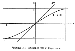
Finally, $b$ must be chosen to attain the desired limits on $s$, so $S(b)=z$ defines $b$ in terms of given $z$. We do not need the explicit expression. The result is an S-shaped curve, with slope

$$S'(x)=1-\frac{e^{\beta x}-e^{-\beta x}}{e^{\beta b}-e^{-\beta b}}$$

Note that the function $\exp(\beta x)+\exp(-\beta x)$ is symmetric and convex. Its minimum occurs at $x=0$, the minimum value being 2. Therefore (i) $S’(0)$ lies between $0$ and $1$, and (ii) $S’(x)$ goes to $0$ as $x$ goes to $\pm b$. Then the function $S(x)$ giving the exchange rate in terms of the fundamental is S-shaped, and everywhere flatter than 1.

Transitional boundary

Sometimes the process encounter not a barrier, but a point of transition where either the parameters of the process, or the flow payoff function, or both, undergo a change. Let $b$ be such a point of transition, and suppose

$$\begin{aligned} \mu & =\mu{1},\ \sigma=\sigma{1},\ f(x)=f_{1}(x)\ when\ x<b \\ \mu & =\mu{2},\ \sigma=\sigma{2},\ f(x)=f_{2}(x)\ when\ x>b \\ \end{aligned}$$

We can use separate differential equations like (19) on each side of $b$ and obtain solutions $F_{1}(x)$ and $F_{2}(x)$. The former is valid for $-\infty<x<b$, and the latter for $b<x<\infty$. Asymptotic considerations allow us to get rid of the term in $\exp(-\alpha_{1}x)$ from $F_{1}(x)$, and that in $\exp(\beta_{2}x)$ from $F_{2}(x)$, where $-\alpha,\beta$ denote the roots of the fundamental quadratic in the respective regious $i=1,2$. Note that $F_{1}(x)$ has no relevance to the right of $b$, so we cannot use the limiting consideration as $x$ goes to $\infty$ for $F_{1}(x)$. Similarly $F_{2}(x)$ cannot be made to satisfy any asymptotic regularity requirement as $x\rightarrow-\infty.$ Therefore each of $F_{1}(x)$ and $F_{2}(x)$ still contains one constant to be determined.

The condition that fixes the two remaining constants is that $F_{1}(x)$ and $F_{2}(x)$ should meet tangentially, or be ’smoothly pasted’ together, at $b$. Thus

$$F_{1}(b)=F_{2}(b),\ F_{1}'(b)=F_{2}'(b)$$

Example: temporary suspension

Return to the firm just above, with two modifications. First, we remove the imposed pricing ceiling. Second, and more important for the current context, we now follow McDonald and Siegel (1985), and let the firm suspend operations when $P<W$.

Now the flow of profits $g(P)$ ha the piecewise linear form

$$g(P)=\begin{cases} 0 & P<W\\ P-W & W<P \end{cases}$$

The differential equation for $G(P)$ correspondingly has two different forms in the two regions. Let $G_{1}(P)$ be the solution in the region $P<W$ and $G_{2}(P)$ that in the region $W<P$. We have

$$G_{1}(P)=D_{1}P^{\delta}$$

and

$$G_{2}(P)=C_{2}P^{-\gamma}+P/(\rho-v)-W/\rho$$

Here we have used two limiting arguments: one as $P$ goes to zero to eliminate the $P^{-\gamma}$ term in $G_{1}(P)$ and the other as $P$ goes to $\infty$ to eliminate the $P^{\delta}$ term in $G_{2}(P)$.

That still leaves two unkown constants. To determine them, we have the value matching and smooth pasting conditions of (3.12) namely

$$\begin{aligned} D{1}W^{\delta} & =C{2}W^{-\gamma}+W/(\rho-v)-W/\rho\\ \delta D{1}W^{\delta-1} & =-\gamma C{2}W^{-\gamma-1}+1/(\rho-v)\end{aligned}$$

These are two simple linear equations for $D_{1}$ and $C_{2}$, which yield

$$D_{1}=\frac{(\rho+\gamma v)W^{1-\delta}}{\rho(\rho-v)(r+\delta)},\ \ C_{2}=\frac{(\rho-\delta v)W^{1+\gamma}}{\rho(\rho-v)(\gamma+\delta)}$$

To find the sign of $C_{2}​$, observe that

$$\begin{aligned} \psi(\rho/v) & =\rho-v(\rho/v)-\frac{1}{2}\sigma^{2}(\rho/v)(\rho/v-1)\\ & =-\frac{1}{2}\sigma^{2}\rho(\rho-v)/v^{2}<0\end{aligned}$$

Therefore $\rho/v$ lies to the right of the root $\delta$ of the fundamental quadratic, or $(\rho-\delta v)$ is positive. Then $C_{2}$ is positive. (A similar calculation shows that $D_{1}$ is positive;). Now we can compare $C_{2}(P)$ in (43) with $G_{0}(P)$ in (35). The latter was the expected present value of the firm’s profits when it was forbidden to shut down. We see how the added term in $G_{2}(P)$ reflects the added benefit of the ability to suspend operations. The benefit is positive even when $P>W$, that is even when the suspension option is not currently being used, becaue there is a positive probability that it will be invoked in the future. But the added value goes to $0$ as $P$ goes to $\infty$, because the nshutdown becomes a remote and unlikely event.

¹. Just recall math textbook introduction of the general solution for ordinary differential equation ↩